一、瞬时功率

$$ p = vi \\\ \\ v = V_mcos(\omega t + \theta_{v}) \\\ \\ i = I_mcos(\omega t + \theta_i) \\\ \\ 更换时刻，可以得到 \\\ \\ v = V_m cos(\omega t + \theta_v - \theta_i) \\\ \\ i = I_mcos\omega t \\\ \\ \therefore p = vi =V_mI_m cos(\omega t + \theta_v - \theta_i)cos\omega t \\\ \\ 根据积化和差与和差化积公式 \\\ \\ p =\frac{V_mI_m}{2}cos(\theta_v - \theta_i) + \frac{V_mI_m}{2} cos(\theta_v - \theta_i)cos2\omega t - \frac{V_mI_m}{2}sin(\theta_v - \theta_i)sin2\omega t [1] $$

二、平均功率与无功功率

2.1 定义

$$ 上述[1]式中 \\\ \\ 令 P = \frac{V_mI_m}{2}cos(\theta_v -\theta_i )， Q = \frac{V_mI_m}{2} sin(\theta_v-\theta_i) \\\ \\ 其中,P = \frac{1}{T} \int_{t_0}^{t_0+T} pd\tau 被称为平均功率\\\ \\ Q被称为无功功率 \\\ \\ 这样一来，p = P + Pcos2\omega t -Qsin2\omega t $$

2.2 纯电阻电路的功率

$$ p = P + Pcos2\omega t \\\ \\ 此时，无功功率为0 $$

2.3 纯电感电路的功率

$$ 电压和电流的相位差为90^{\circ}，即\theta_v-\theta_i = 90^{\circ}\\\ \\ p = -Qsin2\omega t \\\ \\ \pmb{纯电感电路的电路的平均功率为0} \\\ \\ $$

2.4 纯电容电路

$$ 电流超前电压90^{\circ} ，即\theta_v- \theta_i = - 90^{\circ}\\\ \\ p = -Qsin2\omega t \\\ \\ 同样，平均功率为0 $$

2.5 功率因数

$$ 功率因数 pf = cos(\theta_v - \theta_i) \\\ \\ 无功因数 rf(reactive \ factor) = sin(\theta_v - \theta_i) $$

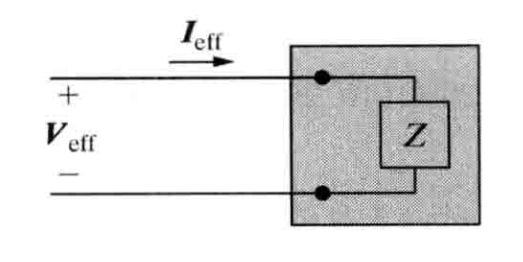
三、均方根和功率计算

$$ 平均功率 P = \frac{1}{T}\int_{t_0}^{t_0+T}\frac{V_m^2cos^2(\omega t + \phi_v)}{R}dt = \frac{1}{R}\Big[\frac{1}{T}\int_{t_0}^{t_0+T}V_m^2cos^2(\omega t + \phi_v)dt\Big] \\\ \\ 根据均方根公式 \\\ \\ 我们知道P = \frac{V_{rms}^2}{R} = I_{rms}^2R\\\ \\ P = V_{eff}I_{eff}cos(\theta_v - \theta_i) \\\ \\ Q = V_{eff}I_{eff}sin(\theta_v - \theta_i) $$

四、复功率

4.1 功率三角形

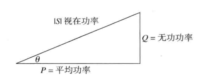
4.2定义

$$ S = P + jQ \\\ \\ tan(\theta_v -\theta_i) = \frac{Q}{P} = tan\theta\\\ \\ |S| = \sqrt{P^2 + Q^2} $$

五、功率计算

$$ S = P + jQ \\\ \\ 经过推导：S = V_{eff}I_{eff}e^{j(\theta_v-\theta_i)} [1]\\\ \\ 也可以变为: S = V_{eff}I_{eff} e^{j(\theta_v - \theta_i)} = V_{eff}e^{j\theta_v} \cdot I_{eff}e^{-j\theta_i} \\\ \\ S = \pmb V_{eff}\cdot \pmb I^{}_{eff}[2] \\\ \\ 其中，I^{eff}是I{eff}的共轭复数 \\\ \\ 同时S = \frac{1}{2}VI [3] $$

5.1 复功率的变换形式

5.1.1 图示

5.1.2 推导

$$ \pmb V_{eff} = \pmb I_{eff}\cdot Z \\\ \\ = \pmb I_{eff}(R+jX) \\\ \\ \therefore S = \pmb{V_{eff}I^*{eff}} \\\ \\ = |\pmb{I{eff}^2}| (R+jX) \\\ \\ = |\pmb{I_{eff}^2}|R+j|\pmb{I_{eff}^2}|X\\\ \\ \therefore P = |\pmb{I_{eff}^2}|R = \frac{1}{2}I_m^2R \\\ \\ Q = |\pmb{I_{eff}^2}|X = \frac{1}{2}I_m^2X $$

5.2 最大功率传输定律

5.2.1 图示

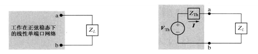
5.2.2 推导

$$ \pmb I = \frac{V_{Th}}{R_{Th}+R_L+j(X_{Th}+X_L)} \\\ \\ P_L = \pmb I^2 \cdot R \\\ \\ \pmb P_L = \frac{V_{Th}^2}{(R_{Th}+R_L)^2+(X_{Th}+X_L)^2} \\\ \\ 通过求导分析可得 \\\ \\ \pmb{当Z_L = Z^*{Th}时，负载功率最大} \\\ \\ 此时\pmb{P{max} = \frac{1}{4}\frac{V_{Th}^2}{R_L} = \frac{1}{8}\frac{V_m^2}{R_L}} $$

5.2.3 限制Z时的最大功率传输

$$ |Z_L| = |Z_{Th}|时,负载平均功率最大 $$