Maxwell Equation & Fields
Maxwell Equation
Differetial Form
$$ \begin{gather} \begin{aligned} \nabla \times \overset{ \longrightarrow }{ \varepsilon} &= - \frac{ \partial \pmb{ B } }{ \partial t } - \pmb{ M } \\ \nabla \times \overset{ \longrightarrow }{ H} &= \frac{ \partial \pmb{ D } }{ \partial t } + \pmb{ J } \\ \nabla \cdot \overset{ \longrightarrow }{ \varepsilon} &= \rho \\ \nabla \cdot \overset{ \longrightarrow }{ H} &= 0 \end{aligned} \end{gather} $$
Integral Form
$$ \begin{gather} \begin{aligned} \oint_{ }^{ } \overrightarrow { \varepsilon} d \overrightarrow{l} &= - \frac{ \partial }{ \partial t } \int_{ }^{ } \pmb{ B } d \overrightarrow{S} - \int_{ }^{ } \pmb{ M } d \overrightarrow{S} \\ \oint_{ }^{ } \overrightarrow { H} d \overrightarrow{l} &= \frac{ \partial }{ \partial t } \int_{ }^{ } \pmb{ D } d \overrightarrow{S} + I \\ \int_{ }^{ } \overrightarrow{ \varepsilon } d \overrightarrow{ S } &= \int_{ }^{ } \rho dV \\ \int_{ }^{ } \overrightarrow{ H} d \overrightarrow{ S } &= 0 \end{aligned} \end{gather} $$
Fields
Average & RMS Electric Field
$$ \begin{gather} \begin{aligned} |\overline{\varepsilon}|^2_{avg} &= \frac{ 1 }{ T } \int_{ 0 }^{ T } \overline{ \varepsilon } \cdot \overline{ \varepsilon } dt \\ &= \frac{ 1 }{ 2 }(E_x^2 + E_y^2 + E_z^2) \\ &= \frac{ 1 }{ 2 } | \overrightarrow{ E }|^2 \\ | \varepsilon|_{rms} &= \frac{ 1 }{ \sqrt{ 2 } } | \overrightarrow{ E }| \end{aligned} \end{gather} $$
Electric Polarization & Electrical Susceptibility
Polarization & Susceptibility & Displacement Current
$$ \begin{gather} \begin{aligned} \overrightarrow{ P_e } &= \epsilon_0 \chi_e \overrightarrow{ E } \\ \overrightarrow{ D } &= \epsilon_0 \overrightarrow{ E } + \overrightarrow{ P_e } \\ &= \epsilon_0 (1 + \chi_e) \overrightarrow{ E } \\ &= \epsilon \overrightarrow{ E } \end{aligned} \end{gather} $$
Permittivity
$$ \begin{gather} \begin{aligned} \epsilon’ &= \epsilon_0 \epsilon_r \\ \epsilon &= \epsilon’ - j \epsilon’’ \\ &= \epsilon_0 \epsilon_r ( 1 - j tan \delta ) \end{aligned} \end{gather} $$
Conducting Current Density
$$ \begin{gather} \begin{aligned} \overrightarrow{ J } &= \sigma \overrightarrow{ E } \end{aligned} \end{gather} $$
Maxwell Equation & Loss Tangent
$$ \begin{gather} \begin{aligned} \nabla \times \overrightarrow{ H } &= j \omega \overrightarrow{ D } + \overrightarrow{ J } \\ &= j \omega \epsilon \overrightarrow{ E } + \sigma \overrightarrow{ E } \\ &= j \omega \epsilon’ \overrightarrow{ E } + ( \omega \epsilon’’ + \sigma) \overrightarrow{ E } \\ &= j \omega \Big[ \epsilon - j ( \epsilon’’ + \frac{ \sigma }{ \omega }) \Big] \overrightarrow{ E } \\ tan \delta &= \frac{ \omega \epsilon’’ + \sigma }{ \omega \epsilon’ } \end{aligned} \end{gather} $$
For Isotropic Materials
$$ \begin{gather} \begin{aligned} [D] &= [\epsilon] [E] \end{aligned} \end{gather} $$
Fields at a General Material Surface
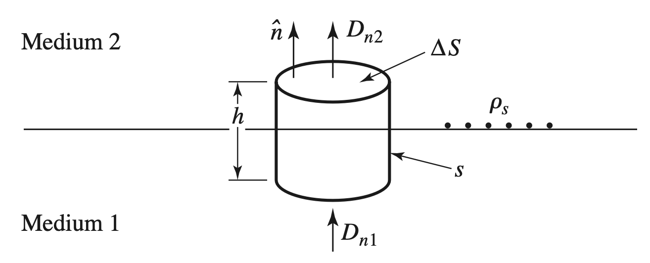
$$ \begin{gather} \begin{aligned} \oint_{ S }^{ } \overrightarrow{ D } \cdot d \overrightarrow{ S } &= \int_{ V }^{ } \rho \ dV \\ (D_{n2} - D_{1n}) \Delta S &= \Delta S \rho_s \\ \therefore \rho_s &= D_{2n} - D_{1n} \end{aligned} \end{gather} $$
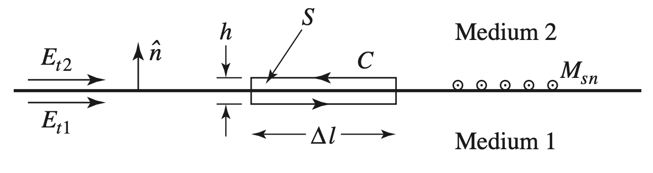
$$ \begin{gather} \begin{aligned} \oint_{ C }^{ } \overrightarrow{ E } \cdot d \overrightarrow{ l } &= - j \omega \int_{ }^{ } \overrightarrow{ B } d \overrightarrow{ S } - \int_{ }^{ } \overrightarrow{ M } d \overrightarrow{ S } \\ (E_{t1} - E_{t2}) \Delta l&= - \Delta l M_s \\ E_{t1} - E_{t2} &= - M_s \end{aligned} \end{gather} $$
Fields at Dielectric Interface
$$ \begin{gather} \begin{aligned} \overrightarrow{ n } \cdot \overrightarrow{ D }_1 &= \overrightarrow{ n } \cdot \overrightarrow{ D }_2 \\ \overrightarrow{ n } \cdot \overrightarrow{ B }_1 &= \overrightarrow{ n } \cdot \overrightarrow{ B}_2 \\ \overrightarrow{ n } \times \overrightarrow{ E_1 } &= \overrightarrow{ n } \times \overrightarrow{ E_2 } \\ \overrightarrow{ n } \times \overrightarrow{ H_1 } &= \overrightarrow{ n } \times \overrightarrow{ H_2 } \end{aligned} \end{gather} $$
Wave Equation
Wave Equations & Basic Plane Wave Solutions In Free Space
Wave Equations
- Maxwell Equation in Frequency Domain & Lossless Medium
$$ \begin{gather} \begin{aligned} \nabla \times \overrightarrow{ E } &= - j \omega \mu \overrightarrow{ H } \\ \nabla \times \overrightarrow{ H } &= j \omega \varepsilon \overrightarrow{ E } \end{aligned} \end{gather} $$
- Mathmatical Transformation
$$ \begin{aligned} \nabla \times \nabla \times \overrightarrow{ E } &= - j \omega \mu \nabla \times \overrightarrow{ H } \\ \nabla ( \nabla \cdot \overrightarrow{ E }) - \nabla^2 \overrightarrow{ E } &= \omega^2 \mu \varepsilon \overrightarrow{E } \end{aligned} $$
- Wave Equations
$$ \begin{gather} \begin{aligned} \nabla^2 \overrightarrow{ E } + k^2 \overrightarrow{ E } &= 0 \\ \nabla^2 \overrightarrow{ H } + k^2 \overrightarrow{ H } &= 0 \\ k &= \omega \sqrt{ \mu \varepsilon } \end{aligned} \end{gather} $$
Basic Plane Wave Solutions in Lossless Medium
假设$\overrightarrow{ E }$只有$x$方向上的分量,且$\dfrac{ \partial }{ \partial x } = \dfrac{ \partial }{ \partial y } = 0$
- Electric Solution
$$ \begin{gather} \begin{aligned} \frac{ \partial^2 E_x }{ \partial z^2 } + k^2 E_x &= 0 \end{aligned} \end{gather} $$
$$ \begin{gather} \begin{aligned} E_x &= E^+ e^{-j k z} + E^- e^{jkz} \end{aligned} \end{gather} $$
- Phase Velocity
$$ \begin{gather} \begin{aligned} \varepsilon_x &= \mathcal{Re} \Big\lbrace E_x e^{j \omega t} \Big\rbrace \\ &= E^+ cos( \omega t - kz) + E^- cos( \omega t + kz) \end{aligned} \end{gather} $$
- 对于特定时间和地点,$\omega t - kz$是常数
$$ \begin{gather} \begin{aligned} v_p &= \frac{ dz }{ dt } = \frac{ \omega }{ k } = \lambda f = \sqrt{ \mu \varepsilon } \end{aligned} \end{gather} $$
- Magenetic Solution
- 将公式(6)代入公式(3)
$$ \begin{gather} \begin{aligned} H_y &= \frac{ 1 }{ \eta } (E^+ e^{-jkz} - E^-e^{j k z}) \\ \eta &= \sqrt{ \frac{ \mu }{ \varepsilon } } \end{aligned} \end{gather} $$
Basic Plane Wave Solutions in Lossy Medium
- Maxwell Equation in Frequency Domain & Lossy Medium
$$ \begin{gather} \begin{aligned} \nabla \times \overrightarrow{ E } &= -j \omega \mu \overrightarrow{ H } \\ \nabla \times \overrightarrow{ H } &= j \omega \epsilon \overrightarrow{ E } + \sigma \overrightarrow{ E } \end{aligned} \end{gather} $$
- Wave Equations
$$ \begin{gather} \begin{aligned} \frac{ \partial^2 E_x }{ \partial z^2 } - \gamma^2 E_x &= 0 \\ \gamma &= \alpha + j \beta = j \omega \sqrt{ \mu \epsilon } \sqrt{ 1- j \frac{ \sigma }{ \omega \epsilon } } \end{aligned} \end{gather} $$
- Solutions
$$ \begin{gather} \begin{aligned} E_x &= E^+ e^{ -\gamma z} + E^- e^{\gamma z} \\ H_y &= \frac{ 1 }{ \eta } (E^+ e^{- \gamma z} - E^- e^{ \gamma z}) \\ \eta &= \frac{ j \omega \mu }{ \gamma } \end{aligned} \end{gather} $$
General Plane Wave Solutions
Wave Equation in General Form
$$ \begin{gather} \begin{aligned} \nabla^2 \overrightarrow{ E } + k_0^2 \overrightarrow{ E } &= 0 \\ \frac{ \partial^2 E_i }{ \partial x^2} + \frac{ \partial^2 E_i }{ \partial y^2 } + \frac{ \partial^2 E_i }{ \partial z^2 } + k_0^2 E_i&= 0 \end{aligned} \end{gather} $$
Considering the X Direction First
- Seperation Variables
$$ \begin{gather} \begin{aligned} E_x(x,y,z) &= f(x) g(y) h(z) \\ f^{’’} gh + fg^{’’} h + fgh^{’’} + k_0^2 fgh &= 0 \\ \frac{ f^{’’} }{ f } + \frac{ g^{’’} }{ g } + \frac{ h^{’’} }{ h } + k_0^2 &= 0 \end{aligned} \end{gather} $$
- 设$\dfrac{ f^{’’} }{ f } = -k_x^2, \dfrac{ g^{’’} }{ g } = - k_y^2, \dfrac{ h^{’’} }{ h } = -k_z^2$
$$ \begin{gather} \begin{aligned} k_x^2 + k_y^2 + k_z^2 &= k_0^2 \end{aligned} \end{gather} $$
- 为了简化情况,先只考虑正向传播, 不考虑反向传播
$$ \begin{gather} \begin{aligned} E_x(x,y,z) &= Ae^{-j(k_x x + k_y y + k_z z)} \\ \overrightarrow{ k } &= k_x \overrightarrow{ x } + k_y \overrightarrow{ y } + k_z \overrightarrow{ z } = k_0 \overrightarrow{ n }\\ \overrightarrow{r} &= x \overrightarrow{ x } + y \overrightarrow{ y } + z \overrightarrow{ z } \\ E_x(x,y,z) &= A e^{- j \overrightarrow{ k } \cdot \overrightarrow{ r }} \end{aligned} \end{gather} $$
- 在计算$k$时, 要考虑电场在各个方向上的分量
Considering All Directions
- Assumptions
$$ \begin{gather} \begin{aligned} E_x(x,y,z) &= A e^{- j \overrightarrow{ k } \cdot \overrightarrow{ r }} \\ E_y(x,y,z) &= B e^{- j \overrightarrow{ k } \cdot \overrightarrow{ r }} \\ E_z(x,y,z) &= C e^{- j \overrightarrow{ k } \cdot \overrightarrow{ r }} \\ \overrightarrow{ E_0 } &= A \overrightarrow{ x } + B \overrightarrow{ y } + C \overrightarrow{ z } \end{aligned} \end{gather} $$
- General Wave Equation Solutions
$$ \begin{gather} \begin{aligned} \overrightarrow{ E } &= \overrightarrow{ E_0 } e^{- j \overrightarrow{ k } \cdot \overrightarrow{ r } } \\ \overrightarrow{ \varepsilon } (x,y,z,t) &= \overrightarrow{ E_0 } \cdot cos( \overrightarrow{ k } \cdot \overrightarrow{ r } - \omega t)\\ \overrightarrow{ H } &= \frac{ j }{ \omega \mu } \nabla \times \overrightarrow{ E } \\ &= \frac{ j }{ \omega \mu } \nabla \times \overrightarrow{ E_0} e^{-j \overrightarrow{ k } \cdot \overrightarrow{ r }} \\ &= - \frac{ j }{ \omega \mu } \overrightarrow{ E_0 } \times \nabla e^{-j \overrightarrow{ k } \cdot \overrightarrow{ r }} \\ &= \frac{ -j }{ \omega \mu } \overrightarrow{ E_0 } \times (-j \overrightarrow{ k }) e^{-j \overrightarrow{ k } \cdot \overrightarrow{ r }} \\ &= \frac{ \overrightarrow{ k } }{ \omega \mu } \times \overrightarrow{ E_0 } e^{-j \overrightarrow{ k } \cdot \overrightarrow{ r }} \\ &= \frac{ 1 }{ \eta } \overrightarrow{ n } \times \overrightarrow{ E } \end{aligned} \end{gather} $$
- Considering Free-Space
$$ \begin{aligned} \nabla \times \overrightarrow{ E} &= 0 \\ -j \overrightarrow{ k } \cdot \overrightarrow{ E_0 } e^{-j \overrightarrow{ k } \cdot \overrightarrow{ r }} &= 0 \end{aligned} $$
$$ \begin{gather} \begin{aligned} \overrightarrow{ k } \cdot \overrightarrow{ E_0 } &= 0 \end{aligned} \end{gather} $$
- 因此,电场方向和电磁波传播方向相互垂直
含义解释
| Category | Concept |
|---|---|
| $\overrightarrow{ E_0 }$ | Electric Field Amplitude Vector |
| $\overrightarrow{ k }$ | Direction of Propogation |
Plane Waves in a Good Conductor
| Good Conductor | Concept |
|---|---|
| 导体电流 » 位移电流 | $\sigma \gg \omega \epsilon$ |
| 能量损失小 | $\epsilon’ \gg \epsilon’'$ |
Complex Propogation Constant
$$ \begin{gather} \begin{aligned} \gamma &= \alpha + j \beta \\ &= j \omega \sqrt{ \mu \epsilon } \sqrt{ 1 - j \frac{ \sigma }{ \omega \epsilon } } \\ & \approx j \omega \sqrt{ \mu \epsilon } \sqrt{ \frac{ \sigma }{ j \omega \epsilon } } \\ &= (1 + j) \sqrt{ \frac{ \omega \mu \sigma }{ 2 } } \end{aligned} \end{gather} $$
Skin Depth
$$ \begin{gather} \begin{aligned} e^{- \alpha z} &= e^{- \alpha \delta_s} = e^{-1} \\ \therefore \delta_s &= \frac{ 1 }{ \alpha } = \sqrt{ \frac{2}{ \omega \mu \sigma } } \end{aligned} \end{gather} $$
定义为电场强度衰减为原来的$e^{-1}$时的深度
Energy and Power
Time-Average Stored Electric & Magenetic Energy
$$ \begin{gather} \begin{aligned} W_e &= \frac{ 1 }{ 4 } \mathcal{Re} \int_{ V }^{ } \overrightarrow{ E } \cdot \overrightarrow{ D }^* dV \\ &= \frac{ \epsilon }{ 4} \int_{ V }^{ } \overrightarrow{ E } \cdot \overrightarrow{ E }^* dV \\ W_m &= \frac{ \mu }{ 4 } \int_{ V }^{ } \overrightarrow{ H } \cdot \overrightarrow{ H }^* dV \end{aligned} \end{gather} $$
Poynting Theorem
Current
- $\overrightarrow{J} = \overrightarrow{ J_s } + \sigma \overrightarrow{ E }$ (电流 = Conduction Current + Source Current)
$$ \begin{aligned} \overrightarrow{ H }^* \cdot ( \nabla \times \overrightarrow{ E }) &= -j \omega \mu | \overrightarrow{ H }|^2 - \overrightarrow{ M } \cdot \overrightarrow{ H }^* \\ \overrightarrow{ E } \cdot ( \nabla \times \overrightarrow{ H }^) &= \overrightarrow{ E } \cdot ( - j \omega \epsilon^ \overrightarrow{ E }^* + \overrightarrow{ J }^) \\ &= -j \omega \epsilon^ | \overrightarrow{ E }|^2 + \overrightarrow{ J_s }^* \cdot \overrightarrow{ E } + \sigma | \overrightarrow{ E }|^2\\ &= ( \sigma - j \omega \epsilon^) | \overrightarrow{ E }|^2 + \overrightarrow{ J_s }^ \cdot \overrightarrow{ E }\\ \therefore \nabla \cdot (\overrightarrow{ E } \times \overrightarrow{ H }^) &= \overrightarrow{ H }^ \cdot ( \nabla \times \overrightarrow{ E }) - \overrightarrow{ E } \cdot ( \nabla \times \overrightarrow{ H }^) \\ &= - \sigma | \overrightarrow{ E }|^2 + j \omega( \epsilon^| \overrightarrow{ E }|^2 - \mu | \overrightarrow{ H }|^2 ) - ( \overrightarrow{ M } \cdot \overrightarrow{ H^* } + \overrightarrow{ J_s }^* \cdot \overrightarrow{ E }) \end{aligned} $$
Gauss’s Law
$$ \begin{aligned} \int_{ V }^{ } \nabla \cdot (\overrightarrow{ E } \times \overrightarrow{ H }^) dV &= \int_{ V }^{ } - \sigma | \overrightarrow{ E }|^2 + j \omega( \epsilon^| \overrightarrow{ E }|^2 - \mu | \overrightarrow{ H }|^2 ) - ( \overrightarrow{ M } \cdot \overrightarrow{ H^* } + \overrightarrow{ J_s }^* \cdot \overrightarrow{ E }) dV \\ \oint_{ }^{ } \overrightarrow{ E } \times \overrightarrow{ H }^* dS &= \int_{ V }^{ } - \sigma | \overrightarrow{ E }|^2 + j \omega( \epsilon^| \overrightarrow{ E }|^2 - \mu | \overrightarrow{ H }|^2 ) - ( \overrightarrow{ M } \cdot \overrightarrow{ H^ } + \overrightarrow{ J_s }^* \cdot \overrightarrow{ E }) dV \end{aligned} $$
考虑介质
-
引入$\epsilon = \epsilon’ - j \epsilon’’, \mu = \mu’ - j \mu’'$
-
Complex Power $P_s$
$$ \begin{gather} \begin{aligned} P_s &= - \frac{ 1 }{ 2 } \int_{ V }^{ } ( \overrightarrow{ E } \cdot \overrightarrow{ J_S }^* + \overrightarrow{ H }^* \times \overrightarrow{ M })dV \\ &= \frac{ 1 }{2 } \oint_{ }^{ }\overrightarrow{ E } \times \overrightarrow{ H }^* d \overrightarrow{ S } + \frac{ \sigma }{ 2 } \int_{ V }^{ } |\overrightarrow{ E }|^2 dV + \frac{ \omega }{2 }\int_{ V }^{ } ( \epsilon’’ | \overrightarrow{ E }|^2 + \mu’’ | \overrightarrow{ H }|^2) dv + j \frac{ \omega }{ 2 } \int_{ V }^{ }( \mu’ | \overrightarrow{ H }|^2 - \epsilon’ | \overrightarrow{ E }|^2)dv \end{aligned} \end{gather} $$
Poynting Vector
- Expression
$$ \begin{gather} \begin{aligned} \overrightarrow{ S } &= \overrightarrow{ E } \times \overrightarrow{ H }^* \end{aligned} \end{gather} $$
描述了电磁场的能量流密度和方向
- Different Parts of the Output Power
$$ \begin{gather} \begin{aligned} P_o &= \frac{ 1 }{ 2 } \oint_{ }^{ } \overrightarrow{ S } \cdot d \overrightarrow{ s } \\ P_l &= \frac{ \sigma }{ 2 } \int_{ V }^{ } | \overrightarrow{ E }|^2 dv + \frac{ \omega }{ 2} \int_{ V }^{ }( \epsilon’’ | \overrightarrow{ E }|^2 + \mu’’ | \overrightarrow{ H }|^2 )dv \\ P_s &= P_o + P_l + 2j \omega (W_m - W_e) \end{aligned} \end{gather} $$
| Category | Concept |
|---|---|
| $P_o$ | 流出Closed Surface $S$的能量$P_o$ |
| $P_l$ | 在空间$V$内由于各种原因损失的均时功率$P_l$, 又称作Joule’s Law |
| $2j \omega (W_m - W_e)$ | 存储的能量 |
- 源提供的能量 = 离开空间的能量 - 损失的能量 + 存储的能量
Power Absorbed By a Good Conductor
Power
$$ \begin{gather} \begin{aligned} P_o &= \frac{ 1 }{ 2 } \mathcal{Re} \Big\lbrace \int_{ S }^{ } \overrightarrow{ E } \times \overrightarrow{ H }^* \cdot \overrightarrow{ n }ds\Big\rbrace \\ \overrightarrow{ n } \cdot ( \overrightarrow{ E } \times \overrightarrow{ H }^) &= \overrightarrow{ n } \times \overrightarrow{ E } \cdot \overrightarrow{ H }^ = \eta | \overrightarrow{ H }|^2 \\ \therefore P_o &= \frac{ R_s }{ 2 } \int_{ _S }^{ } | \overrightarrow{ H }|^2 ds \end{aligned} \end{gather} $$
Surface Resistance
$$ \begin{gather} \begin{aligned} R_s &= \mathcal{Re} \Big\lbrace \eta \Big\rbrace \\ &= \mathcal{Re} \Big\lbrace (1+j) \sqrt{ \frac{ \omega \mu }{ 2 \sigma} } \Big\rbrace \\ &= \sqrt{ \frac{ \omega \mu }{ 2 \sigma }} \\ &= \frac{ 1 }{ \sigma \delta_s } \end{aligned} \end{gather} $$
Plane Wave Reflection From a Media Interface
General Medium
Incident, Reflected, Transmitted Waves
$$ \begin{gather} \begin{aligned} \overrightarrow{ E_i } &= E_0e^{-jk z} \overrightarrow{ x } \\ \overrightarrow{ H_i } &= \frac{ 1 }{ \eta_0 }E_0e^{-jk z} \overrightarrow{ y} \\ \overrightarrow{ E_r } &= \Gamma E_0 e^{jkz} \overrightarrow{ x } \\ \overrightarrow{ H_r} &= -\frac{ \Gamma }{ \eta_0 }E_0e^{jk z} \overrightarrow{ y} \\ \overrightarrow{ E_t } &= T E_o e^{- \gamma z} \overrightarrow{ x } \\ \overrightarrow{ H_t } &= \frac{ T E_0}{ \eta } e^{- \gamma z} \overrightarrow{ y } \end{aligned} \end{gather} $$
Transmission Coefficient & Reflection Coefficient
$$ \begin{gather} \begin{aligned} \overrightarrow{ E_t } &= \overrightarrow{ E_i } + \overrightarrow{ E_r } \\ \overrightarrow{ H_t } &= \overrightarrow{ H_i } + \overrightarrow{ H_r } \end{aligned} \end{gather} $$
- 在$z=0$时,以上公式成立
$$ \begin{gather} \begin{aligned} 1 + \Gamma &= T \\ \frac{ 1 - \Gamma }{ \eta_0 } &= \frac{ T }{ \eta } \end{aligned} \end{gather} $$
- 解得:
$$ \begin{gather} \begin{aligned} \Gamma &= \frac{ \eta - \eta_0 }{ \eta + \eta_0} \\ T &= \frac{ 2 \eta }{ \eta + \eta_0 } \end{aligned} \end{gather} $$
Lossless Medium
Basic Parameters
$$ \begin{gather} \begin{aligned} \gamma &= j \beta = j k_0 \sqrt{ \mu_r \epsilon_r }, \alpha = 0 \\ v_p &= \frac{ \omega }{ \beta } = \frac{ 1 }{ \sqrt{ \mu \epsilon } } \\ \lambda &= \frac{ 2 \pi }{ \beta } = \frac{ \lambda_0 }{ \sqrt{ \mu \epsilon } } \\ \eta &= \eta_0 \sqrt{ \frac{ \mu_r }{ \epsilon_r } } \end{aligned} \end{gather} $$
Poynting Vectors
$$ \begin{gather} \begin{aligned} \overrightarrow{ S_i } &= \frac{ E_0^2 }{ \eta_0 } \overrightarrow{ z } \\ \overrightarrow{ S_r } &= - \frac{ \Gamma^2 E_0^2}{ \eta_0 } \overrightarrow{ z } \\ \overrightarrow{ S }^- &= ( \overrightarrow{ E_i } + \overrightarrow{ E_r }) \times ( \overrightarrow{ H_i } + \overrightarrow{ H_r })^* \\ &= E_0^2 \frac{ 1 }{ \eta_0 } (1 - \Gamma^2 + 2j \Gamma sin(2 k_0z)) \overrightarrow{ z } \\ \overrightarrow{ S }^+ &= \overrightarrow{ E }_t \times \overrightarrow{ H }^*_t \\ &= \frac{ E_0^2}{ \eta_0 } (1 - \Gamma^2) \overrightarrow{ z } \\ &= \frac{ E_0^2 T^2 }{\eta_0} \overrightarrow{ z } \\ \overrightarrow{ S_i } + \overrightarrow{ S_r } & \neq \overrightarrow{ S }^- \end{aligned} \end{gather} $$
Power Per Unit Area
$$ \begin{gather} \begin{aligned} P^- &= \frac{ 1 }{ 2 } \mathcal{Re} \Big\lbrace \overrightarrow{ S}^- \cdot \overrightarrow{ z } \Big\rbrace = P^+ = \frac{ E_0^2 T^2 }{ \eta_0 } \end{aligned} \end{gather} $$
- 因此,实部功率没有损失
Good Conductor
Poynting Vectors & Power
$$ \begin{gather} \begin{aligned} S^-(z=0) &= \frac{ \overrightarrow{ E } }{ \eta_0 } (1 - | \Gamma|^2 + \Gamma - \Gamma^*) \\ S^+ &= S^-(z=0) e^{-2 \alpha z} \\ \overrightarrow{ S_i} + \overrightarrow{ S_r } &= \overrightarrow{ S }^- \\ \overrightarrow{ P_i} + \overrightarrow{ P_r } &= \overrightarrow{ P }^- \\ P^+ &= P^- \cdot e^{-2 \alpha z} \end{aligned} \end{gather} $$
Dissipated Power & Transmitted Power Per Unit Area
$$ \begin{gather} \begin{aligned} \overrightarrow{ J_t } &= \sigma \overrightarrow{ E_t } \\ &= \sigma T E_0 e^{-2 \gamma z} \overrightarrow{ x } \\ P^t &= \frac{ 1 }{ 2 } \int_{ V }^{ } \overrightarrow{ E } \cdot \overrightarrow{ J_t }^* dV \\ &= \frac{ \sigma }{ 2 } \int_{ x = 0 }^{ 1 } \int_{ y=0 }^{ 1 } \int_{ z=0 }^{ \infin } T^2 E_0^2 e^{-2 \alpha z} \overrightarrow{ x } dzdydx \\ &= \frac{ \sigma |T|^2|E_0|^2 }{ 2 } \int_{ z=0 }^{ \infin }e^{-2 \alpha z} dz \\ &= \frac{ \sigma |T|^2 |E_0|^2 }{ 4 \alpha} \end{aligned} \end{gather} $$
Surface Impedance …
$$ \begin{gather} \begin{aligned} \frac{ \sigma |T|^2 }{ \alpha } &= \frac{ \sigma \delta_s 4 |\eta|^2 }{ ( \eta + \eta_0)^2 } \\ &\approx \frac{ 8 }{ \sigma \delta_s \eta_0^2 } \end{aligned} \end{gather} $$
Perfect Conductor
- 对于$z<0$, $\sigma \longrightarrow \infin, \delta_s \longrightarrow 0, \eta \longrightarrow 0, T=0, \Gamma = -1, \alpha \longrightarrow \infin$
Fields
$$ \begin{gather} \begin{aligned} \overrightarrow{ E } &= \overrightarrow{ E_i } + \overrightarrow{ E_r } \\ &= E_0(e^{-jk_0 z} - e^{j k_0 z}) \overrightarrow{ x } \\ &= -2j E_0 sin(k_0 z) \overrightarrow{ x } \\ \overrightarrow{ H } &= \frac{ 2 }{ \eta_0 } E_0 cos(k_0 z) \overrightarrow{ y } \\ \end{aligned} \end{gather} $$
Power Current
$$ \begin{gather} \begin{aligned} \overrightarrow{ S } &= -j \frac{ 4 }{ \eta_0 } |E_0|^2 sin(k_0z)cos(k_0z) \overrightarrow{ z } \\ \overrightarrow{ J_s } &= \sigma \overrightarrow{ E } \\ &= \eta \sigma \overrightarrow{ n } \times \overrightarrow{ H } \\ &= - \frac{ 2 }{ \eta_0 } E_0 cos(k_0 z) \overrightarrow{ x } \end{aligned} \end{gather} $$
Oblique Incidence at a Dielectric Interface
Parallel Polarization
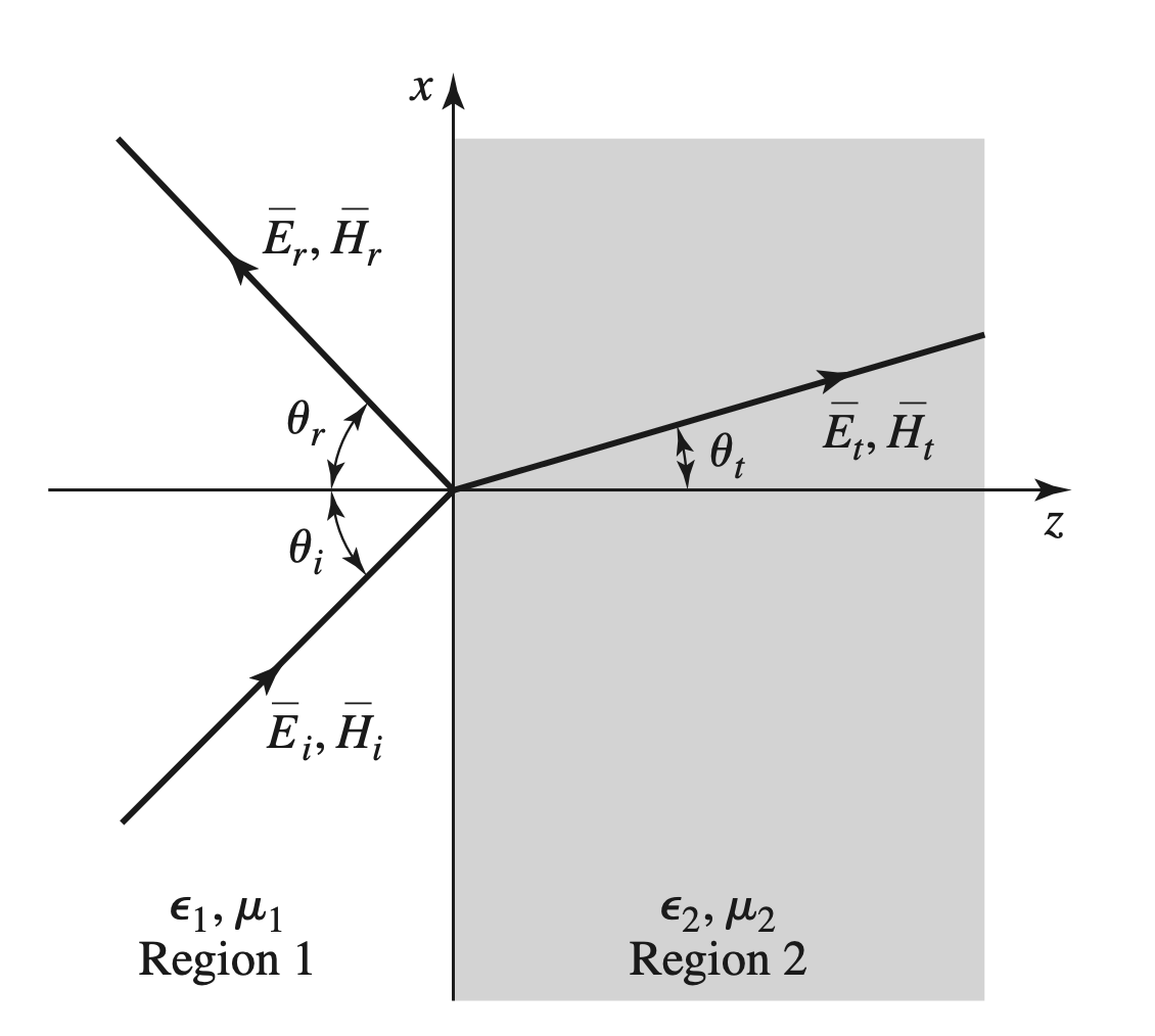
Wave Solutions
$$ \begin{gather} \begin{aligned} \overrightarrow{ E_i } &= E_0 (\overrightarrow{ x } cos \theta_i - \overrightarrow{ z} sin \theta_i) e^{- j k_1 (x \cdot cos \theta_i + z \cdot sin \theta_i)} \\ \overrightarrow{ H_i } &= \frac{ E_0 }{ \eta_1 } \overrightarrow{ y } e^{- j k _1 (x \cdot sin\theta_i + z \cdot cos \theta_i)} \\ \overrightarrow{ E_r } &= \Gamma E_0 (\overrightarrow{ x } cos \theta_r + \overrightarrow{ z} sin \theta_r) e^{- j k_1 (x \cdot cos \theta_r - z \cdot sin \theta_r)} \\ \overrightarrow{ H_r } &= - \frac{ \Gamma E_0 }{ \eta_1 } \overrightarrow{ y } e^{- j k _1 (x \cdot sin\theta_r + z \cdot cos \theta_r)} \\ \overrightarrow{ E_t } &= T E_0 (\overrightarrow{ x } cos \theta_t - \overrightarrow{ z} sin \theta_t) e^{- j k_2 (x \cdot cos \theta_t + z \cdot sin \theta_t)} \\ \overrightarrow{ H_t } &= \frac{ T E_0 }{ \eta_2 } \overrightarrow{ y } e^{- j k_2 (x \cdot sin\theta_t + z \cdot cos \theta_t)} \\ k_1 &= \omega \sqrt{ \mu_0 \epsilon_1 }, \eta_1 = \sqrt{ \frac{ \mu_0 }{ \epsilon_1 }} \\ k_2 &= \omega \sqrt{ \mu_0 \epsilon_2 }, \eta_2 = \sqrt{ \frac{ \mu_0 }{ \epsilon_2 }} \end{aligned} \end{gather} $$
Coefficients
- 结合公式$26,31$, 当$z = 0$时
$$ \begin{gather} \begin{aligned} cos \theta_i e^{-j k_1 x cos \theta_i}+ \Gamma cos \theta_r e^{-jk_1 x cos \theta_r} &= T cos \theta_t e^{-j k_2 cos \theta_t} \\ \frac{ 1 }{ \eta_1 } e^{-j k_1 x \cdot sin \theta_i} - \frac{ \Gamma }{ \eta_1 } e^{-jk_2 x \cdot sin \theta_r} &= \frac{ T}{ \eta_2 } e^{-j k_2 x \cdot sin \theta_t} \end{aligned} \end{gather} $$
- 解得
$$ \begin{gather} \begin{aligned} \Gamma &= \frac{ \eta_2 cos \theta_t - \eta_1 cos \theta_i }{ \eta_2 cos \theta_t + \eta_1 cos \theta_i } \\ T &= \frac{ 2 \eta_2 cos \theta_i }{ \eta_2 cos \theta_t + \eta_1 cos \theta_i } \end{aligned} \end{gather} $$
Snell’s Law & Brewster’s Angle
- 若要在z=0处连续, 可以得到 Snell’s Law
$$ \begin{gather} \begin{aligned} k_1 cos \theta_i &= k_1 cos \theta_r = k_2 sin \theta_t \\ \theta_i &= \theta_r \\ k_1 sin \theta_i &= k_2 sin \theta_t \end{aligned} \end{gather} $$
- Brewster’s Angle
- 当 $\eta_2 cos \theta_t = \eta_1 cos \theta_i$ 时, $\theta_b = \theta_i$
$$ \begin{gather} \begin{aligned} sin \theta_b &= \frac{ 1 }{ \sqrt{ 1 + \epsilon_1/ \epsilon_2 } } \end{aligned} \end{gather} $$
Perpendicular Polarization
Wave Solutions
$$ \begin{gather} \begin{aligned} \overrightarrow{ E_i } &= E_0 \overrightarrow{ y } e^{-j k_1 (x \cdot sin \theta_i + z \cdot cos \theta_i)} \\ \overrightarrow{ H_i } &= \frac{ E_0 }{ \eta_1 } (- \overrightarrow{ x } \cdot cos \theta_i + \overrightarrow{ z } \cdot sin \theta_i) e^{-j k_1 (x \cdot sin \theta_i + z \cdot cos \theta_i)} \\ \overrightarrow{ E_r } &= \Gamma E_0 \overrightarrow{ y } e^{-j k_1 (x \cdot sin \theta_r - z \cdot cos \theta_r)} \\ \overrightarrow{ H_r } &= - \frac{ \Gamma E_0 }{ \eta_1 } ( \overrightarrow{ x } \cdot cos \theta_r + \overrightarrow{ z } \cdot sin \theta_r) e^{-j k_1 (x \cdot sin \theta_r + z \cdot cos \theta_r)} \\ \overrightarrow{ E_t } &= E_0 T \overrightarrow{ y } e^{-j k_1 (x \cdot sin \theta_t - z \cdot cos \theta_t)} \\ \overrightarrow{ H_i } &= \frac{ E_0 T }{ \eta_1 } (- \overrightarrow{ x } \cdot cos \theta_t + \overrightarrow{ z } \cdot sin \theta_t) e^{-j k_1 (x \cdot sin \theta_t + z \cdot cos \theta_t)} \end{aligned} \end{gather} $$
Coefficients
$$ \begin{gather} \begin{aligned} \Gamma &= \frac{ \eta_2 cos \theta_t - \eta_1 cos \theta_i }{ \eta_2 cos \theta_i + \eta_1 cos \theta_t } \\ T &= \frac{ 2 \eta_2 cos \theta_i }{ \eta_2 cos \theta_i + \eta_1 cos \theta_t } \end{aligned} \end{gather} $$
Total Reflection & Surface Wave …
Incident Angle & Reflection Coefficients
- Critical Angle $\theta_c$: 此时$\theta_t = \dfrac{ \pi }{ 2 }$
$$ \begin{gather} \begin{aligned} sin \theta_t &= \sqrt{ \frac{ \epsilon_1 }{ \epsilon_2 } } sin \theta_i \\ sin \theta_c &= \sqrt{ \frac{ \epsilon_2 }{ \epsilon_1 } } \end{aligned} \end{gather} $$
- 对于$\theta_i > \theta_c$, 都会发生完全反射
Some useful Theorems & Appendix
Lorentz Reciprocity Theorem
Statement
- 两个独立源产生电磁场
$$ \begin{gather} \begin{aligned} \nabla \cdot ( \overrightarrow{ E_1 } \times \overrightarrow{ H_2 } - \overrightarrow{ E_2 } \times \overrightarrow{ H_1 }) &= \overrightarrow{ J_1} \cdot \overrightarrow{ E_2 } - \overrightarrow{ J_2 } \cdot \overrightarrow{ E_1 } + \overrightarrow{ M_2 } \cdot \overrightarrow{ H_1 } - \overrightarrow{ M_1 } \cdot \overrightarrow{ H_2 } \\ \oint_{ S }^{ } ( \overrightarrow{ E_1 } \times \overrightarrow{ H_2 } - \overrightarrow{ E_2 } \times \overrightarrow{ H_1 }) d \overrightarrow{ S } &= \int_{ V }^{ }\overrightarrow{ J_1} \cdot \overrightarrow{ E_2 } - \overrightarrow{ J_2 } \cdot \overrightarrow{ E_1 } + \overrightarrow{ M_2 } \cdot \overrightarrow{ H_1 } - \overrightarrow{ M_1 } \cdot \overrightarrow{ H_2 } d \overrightarrow{ V } \end{aligned} \end{gather} $$
In Special Conditions
- S encloses No Sources
$$ \begin{gather} \begin{aligned} \oint_{ S }^{ } \overrightarrow{ E_1 } \times \overrightarrow{ H_2 } d \overrightarrow{ S } &= \oint_{ S }^{ } \overrightarrow{ E_2 } \times \overrightarrow{ H_1 } d \overrightarrow{ S } \end{aligned} \end{gather} $$
- S bounds a Perfect Conductor / S is at Infinity
-
Perfect Conductor
-
S At Infinity, 可以将其视为平面波
$$ \begin{gather} \begin{aligned} \int_{ V } \overrightarrow{ E_1 } \cdot \overrightarrow{ J }2 - \overrightarrow{ H_1 } \cdot \overrightarrow{ M_2 } dV &= \int{ V }\overrightarrow{ E_2 } \cdot \overrightarrow{ J_1 } - \overrightarrow{ H_2 } \cdot \overrightarrow{ M_1} dV \end{aligned} \end{gather} $$
单位换算 公式
$$ \begin{gather} \begin{aligned} \sigma &= \omega \epsilon \Longleftrightarrow \epsilon= \sigma t \\ \overrightarrow{ J } &= \sigma \overrightarrow{ E } = \overrightarrow{ n } \times \overrightarrow{ H} \end{aligned} \end{gather} $$
$$ \begin{gather} \begin{aligned} \overrightarrow{ a } \times \overrightarrow{ a } \times \overrightarrow{ b } &= \overrightarrow{ b } \\ \sqrt{ 2j } &= 1 + j \\ \overrightarrow{ J}_d &= \frac{ d \overrightarrow{ D } }{ d t } \end{aligned} \end{gather} $$