离散时不变系统 - 卷积和
用脉冲表示离散时间信号
$$ \begin{aligned} x[n] &= \sum_{k = -\infin}^{\infin} x[k] \delta[n-k] \\ u[n] &= \sum_{k=0}^{\infin} \delta[n-k] \end{aligned} $$
离散卷积定义
$$ \begin{aligned} y[n] &= \sum_{-\infin}^{\infin}x[k]h[n-k] \end{aligned} $$
连续时不变系统 - 卷积积分
用脉冲表示连续时间信号
$$ \begin{aligned} x(t) &= \int_{-\infin}^{+\infin} x(\tau) h(t-\tau) d\tau \\ u(t) &= \int_{-\infin}^{\infin} \delta(t-\tau) d\tau \end{aligned} $$
连续卷积定义
$$ \begin{aligned} y(t) &= \int_{-\infin}^{\infin} x(\tau)h(t-\tau) d\tau \end{aligned} $$
卷积
数学表示
$$ \begin{aligned} y[n] &= \sum_{ k =-\infin}^{\infin}x[k]h[n-k] = x[n]*h[n] \\ y(t) &= \int_{-\infin}^{\infin} x(\tau)h(t-\tau) d\tau = x(t) * h(t) \\ \end{aligned} $$
性质
Commutative Distributive Associative (交换 分配 结合)
$$ \begin{gather} \begin{aligned} x(t)*h(t) &= h(t)x(t) \\ x(t)[h_1(t) + h_2(t)] &= x(t)*h_1(t) + x(t) * h_2(t) \\ x(t) * h_1(t) * h_2(t) &= x(t) * (h_1(t) * h_2(t)) \end{aligned} \end{gather} $$
其他性质
- 若$y(t) = x(t) * h(t)$
$$ \begin{equation} y(t-k) = x(t-k) * h(t) \end{equation} $$
$$ \begin{equation} y’(t) = x’(t) * h(t) \end{equation} $$
$$ \begin{equation} y(-t) = x(-t) * h(-t) \end{equation} $$
$$ \begin{equation} y(kt) \neq x(kt) * h(t) \end{equation} $$
$$ \begin{equation} x(t) * u(t) = \int_{ - \infin }^{ t } x( \tau) d \tau \end{equation} $$
线性时不变系统(LTI)的性质
| 性质 | 需要满足的方程 | 其他特征 |
|---|---|---|
| Linear | $x_3(t) = Ax_1(t) + Bx_2(t) \Longleftrightarrow y_3(t) = Ay_1(t) + By_2(t)$ | Cascode System的先后位置不重要 |
| Time-Inviriant | $y(t-t_0) = y_1(t) \Longleftrightarrow x_(t-t_0) = x_1(t)$ | |
| MemoryLess | $h[n] = 0, n \neq 0$ | $h[n] = K \delta [n], n =0$ |
| Invertibility | $h[n] * g[n] = \delta [n]$,分别为原、逆系统的UIR | |
| Casuality | $h[n] = 0, n < 0$ | $y[n] = \sum_{ k =0 }^{ \infin } x[n] h[n-k]$ |
| Stability | $\int_{ - \infin }^{ \infin } h( \tau) d \tau < 0$ |
Response of a LTI System
Unit Impulse Response
输入为$\delta (t)$时的输出$h(t)$
- Cascaded System UIR
$$ \begin{equation} h(n) = h_1(n)*h_2(n) \end{equation} $$
Unit Step Response
输入为$u(t)$时的输出$s(t)$
$$ \begin{equation} s[n] = u[n] * h[n] = \sum_{ k = - \infin }^{ n } h[k] \end{equation} $$
$$ \begin{equation} s(t) = u(t) * h(t) = \int_{ - \infin }^{ t } h(\tau) d \tau \end{equation} $$
Casual LTI System Described by LCCDE
- Linear Constant-Coefficient Differential and Difference Equation
一阶线性常微分方程的通用解法
一般形式
$$ \begin{aligned} \sum_{k=0}^N a_k \frac{d^ky}{dt} &= \sum_{k=0}^{M}b_k \frac{d^k x}{dt} \end{aligned} $$
解法
- $N = 0$
$$ \begin{aligned} y(t) &= \sum_{k=0}^{M}b_k \frac{d^k x}{dt} \end{aligned} $$
- $N \ge 1$
- Initial Condition
$$ \begin{aligned} y(t_0) &= \frac{dy(t_0)}{dt} = … = \frac{d^{N-1} y(t_0)}{dt^{N-1}} \end{aligned} $$
一阶线性差分方程
形式 (recursive equations)
$$ \begin{aligned} \sum_{k=0}^N a_k y[n-k] &= \sum_{k=0}^M b_k x[n-k] \\ y[n] &= \frac{1}{a_0}(\sum_{k=0}^M b_k x[n-k] - \sum_{k=1}^N a_k y[n-k]) \end{aligned} $$
解法
- 当 $N=0$, 存在Finite Impulse Response
$$ \begin{aligned} y[n] &= \frac{b_k}{a_0}\sum_{k=0}^{M}x[n-k] \\ h[n] &= \begin{cases} \frac{b_n}{a_0} & 0 \lt n \le M \\ 0 & otherwise \end{cases} \end{aligned} $$
- Infinite Impulse Response Ex.
$$ \begin{aligned} y[n] &= \frac{1}{2} y[n-1] + K \delta[n] \\ \therefore y[n] &= 0, n \le -1 \\ \therefore y[0] &= K \\ y[1] &= \frac{1}{2}K \\ y[2] &= (\frac{1}{2})^2K \\ … \\ y[n] &= (\frac{1}{2})^n K \end{aligned} $$
- 因此,Impulse Response 是 $h[n] = (\dfrac{1}{2})^n u[n]$
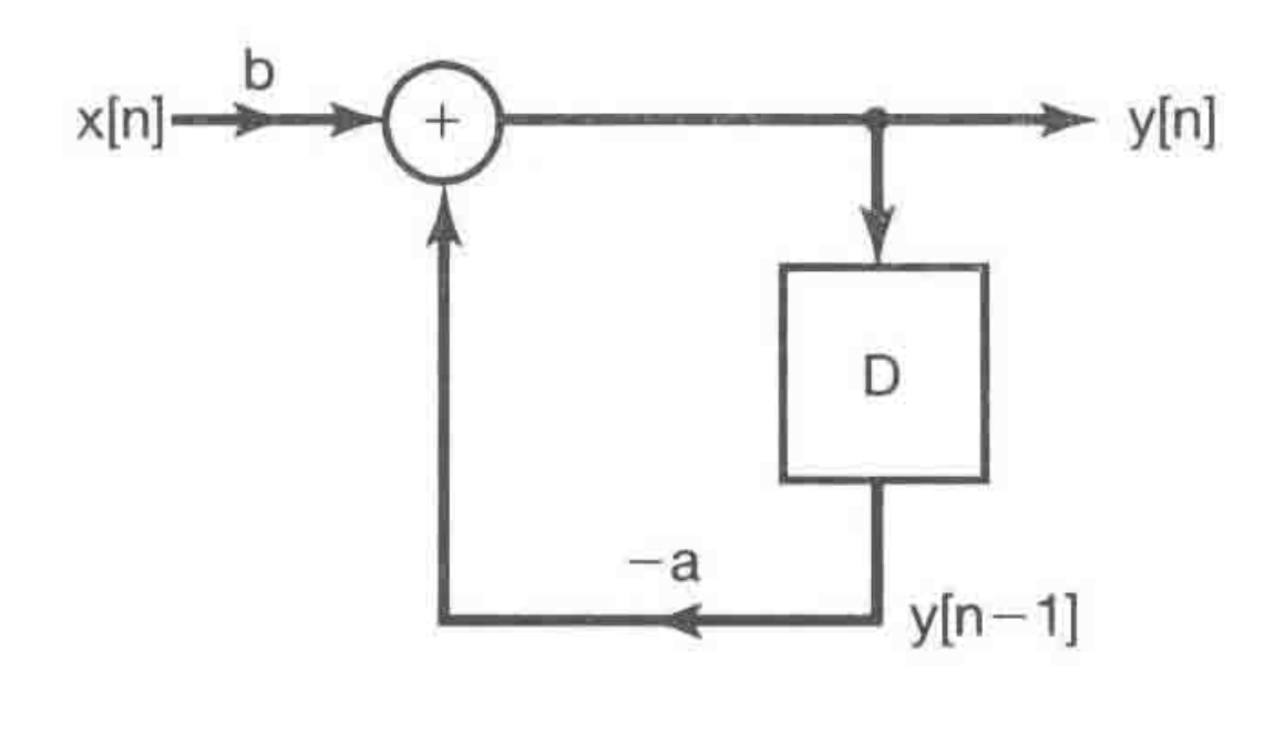
Block Diagram Representations of First-Order Systems Described by Differential and Difference Equations
Difference Equations for Discrete-Time
$$ \begin{aligned} y[n] &= -ay[n-1] + bx[n] \end{aligned} $$
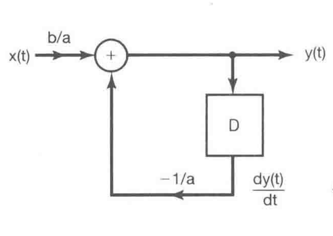
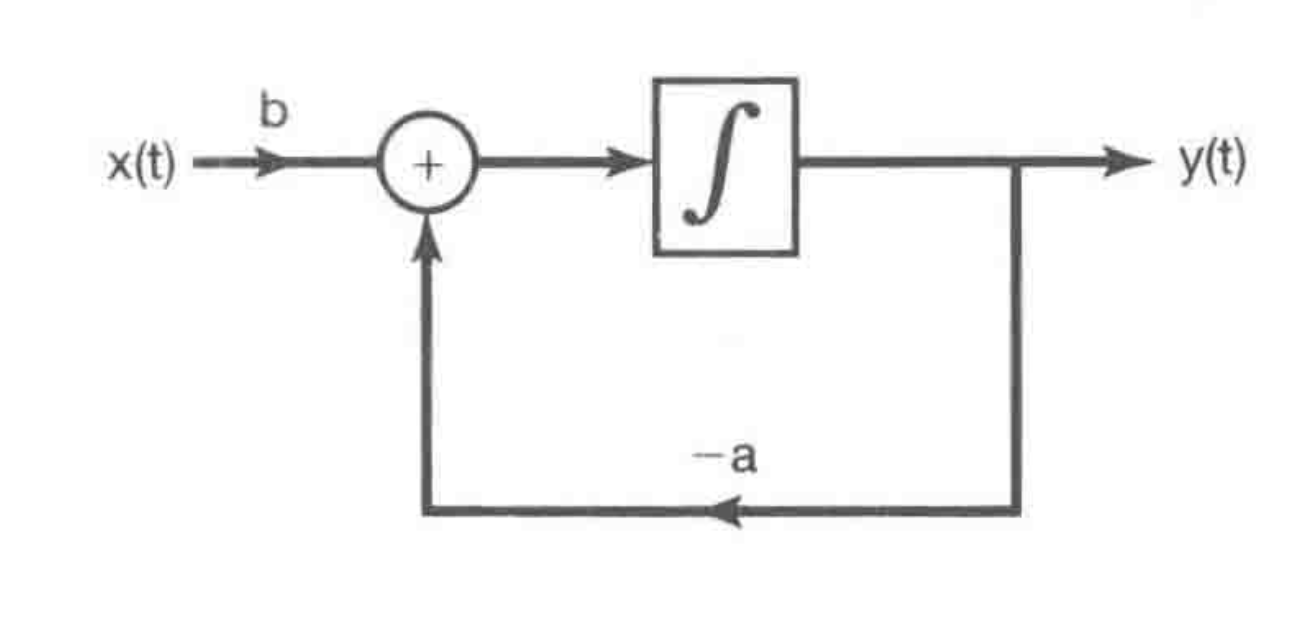
Differential Equations for Continuous-Time
- Block Diagram I
$$ \begin{aligned} \frac{dy(t)}{dx} + a y(t) &= bx(t) \\ \therefore y(t) &= \frac{1}{a} [bx(t) - \frac{dy(t)}{dt}] \end{aligned} $$
- Block Diagram II
$$ \begin{aligned} y(t) &= y(t_0) + \int_{-\infin}^{t} [bx(\tau) - ay(\tau)] d\tau \end{aligned} $$
Singularity Functions
$$ \begin{equation} u_k(t) = \begin{cases} \dfrac{ d^k \delta (t) }{ dt^k } & k > 0 \\ \int_{ - \infin }^{ t } u_{k+1} ( \tau) d \tau & k \le 0 \end{cases} \end{equation} $$
Unit Doublets and other Singularity Functions
$$ \begin{aligned} \frac{dx(t)}{dt} &= x(t) *u_1(t) \\ \frac{d^2x(t)}{dt} &= x(t) * u_2(t) \\ … \\ \therefore u_k(t) &= \underset{k \ times}{u_1(t) * u_1(t) *..*u_1(t)} \end{aligned} $$
微分方程解法回顾
常系数一阶微分方程
形式
$$ \begin{aligned} a \frac{dy(x)}{dx} + b y(x) &= cx \\ y &= y_h(x) + y_p(x) \end{aligned} $$
解法
- $y_h(x)$
- 先将$y_h(x)$设为和$x$相似的形式,再进行如下步骤:
$$ \begin{aligned} Let \ c &= 0 \\ a\frac{dy(t)}{dt} + by(t) &= 0 \Longrightarrow y_h(x) \\ \end{aligned} $$
- $y_p(x)$
- 将$y_p(x)$设为$x$的倍数,再代入解
一阶微分方程
- 形式
$$ \begin{aligned} \frac{dy}{dx} + P(x) y &= Q(x) \\ \end{aligned} $$
- 解法
$$ \begin{aligned}
Let \ v’(x) &= v(x) P(x) \\ \Big[\frac{1}{v(x)} dv &= P(x)dx \Longrightarrow v(x) = e^{\int P(x) dx} \Big]\\ \therefore \frac{dy}{dx} v(x) + P(x)v(x) y &=Q(x) v(x) \\ y v(x) &= \int Q(x)v(x) - P(x) v(x) ydx \\ yv(x) &= \int Q(x) v(x) dx - \int ydv \\ y &= \frac{1}{v(x)} \int Q(x) v(x) dx (????) \end{aligned} $$
常系数二阶微分方程
形式
$$ \begin{aligned} ay’’ + by’ + cy &= 0 \end{aligned} $$
解法
- 换成$ay^2 + by + c = 0$,获得解
| 两个实根 | $y = c_1 e^{r_1x} + c_2 e^{r_2 x}$ |
|---|---|
| 一个实根 | $y = c_1 e^{rx} +c_2 x e^{rx}$ |
| 两个复数根$r = \alpha \pm i \beta$ | $y = e^{\alpha x} (c_1 \cos \beta x + c_2 \sin \beta x)$ |
重要公式
$$ \begin{aligned} \sum_{k=0}^n \alpha^k &= \frac{1 - \alpha^{n+1}}{1 -\alpha} \end{aligned} $$