General Solutions for TEM, TE, TM Waves in Free Space

General Solutions

Equations

• 拆成Transverse Wave和Longitudinal Wave

$$ \begin{gather} \begin{aligned} \overrightarrow{ E }(x,y,z) &= \Big[ \overrightarrow{ e}(x,y) + \overrightarrow{ z } \cdot \overrightarrow{ e }_z (x,y) \Big]e^{-j \beta z} \\ \overrightarrow{ H }(x,y,z) &= \Big[ \overrightarrow{ h}(x,y) + \overrightarrow{ z } \cdot \overrightarrow{ h }_z (x,y) \Big]e^{-j \beta z} \\ \nabla \times \overrightarrow{ E } &= - j \omega \mu \overrightarrow{ H } \\ \nabla \times \overrightarrow{ H } &= -j \omega\mu \overrightarrow{ E } \end{aligned} \end{gather} $$

Maxwell Equations in 3 Directions

$$ \begin{gather} \begin{aligned} \frac{ \partial E_z }{ \partial y } + j \beta E_y &= - j \omega \mu H_x \\

• j \beta E_x - \frac{ \partial E_z }{ \partial x } &= - j \omega \mu H_y \\ \frac{ \partial E_y }{ \partial x } - \frac{ \partial E_x }{ \partial y } &= - j \omega \mu H_z \\ \frac{ \partial H_z }{ \partial y } + j \beta H_y &= j \omega \epsilon E_x \\
• j \beta H_x - \frac{ \partial H_z }{ \partial x } &= j \omega \epsilon E_y \\ \frac{ \partial H_y }{ \partial x } - \frac{ \partial H_x }{ \partial y } &= j \omega \epsilon E_z \end{aligned} \end{gather} $$

Transverse Wave Solutions Using Longitudinal Wave

$$ \begin{gather} \begin{aligned} H_x &= \frac{ j }{ k_c^2 } ( \omega \epsilon \frac{ \partial E_z }{ \partial y } - \beta \frac{ \partial H_z }{ \partial x }) \\ H_y &= \frac{ -j }{ k_c^2 } ( \omega \epsilon \frac{ \partial E_z }{ \partial x } + \beta \frac{ \partial H_z }{ \partial y }) \\ E_x &= \frac{ -j }{ k_c^2 } ( \beta \frac{ \partial E_z }{ \partial x } + \omega \mu \frac{ \partial H_z }{ \partial y }) \\ E_y &= \frac{ j }{ k_c^2 } ( -\beta \frac{ \partial E_z }{ \partial y } + \omega \mu \frac{ \partial H_z }{ \partial x }) \\ k_c^2 &= k^2 - \beta^2 \end{aligned} \end{gather} $$

TEM Waves

Features

$$ \begin{gather} \begin{aligned} E_z &= H_z = 0 \\ \therefore \beta &= k = \omega \sqrt{ \mu \epsilon } \\ k_c &= 0 \end{aligned} \end{gather} $$

Field and Potential

1. Fields

$$ \begin{gather} \begin{aligned} ( \frac{ \partial^2 }{ \partial x^2 } + \frac{ \partial^2 }{ \partial y^2 } + \frac{ \partial^2 }{ \partial z^2 } + k^2) E_x &= 0 \\ ( \frac{ \partial^2 }{ \partial x^2 } + \frac{ \partial^2 }{ \partial y^2 }) E_x &= 0 \\ \nabla^2_t \cdot \overrightarrow{ e } (x,y) &= 0 \\ \therefore \nabla_t^2 \cdot \overrightarrow{ h }(x,y) &= 0 \end{aligned} \end{gather} $$

2. Potential (Laplace Equation)

$$ \begin{gather} \begin{aligned} \overrightarrow{ e } (x,y) &= - \nabla_t \cdot \Phi(x,y) \\ \nabla^2_t \cdot \Phi(x,y) &= 0 \end{aligned} \end{gather} $$

Expression

$$ \begin{gather} \begin{aligned} Z_{TEM} &= \frac{ E_x }{ H_y } = \frac{ -E_y }{ H_x } = \eta \\ \overrightarrow{ h }(x,y) &= \frac{ 1 }{ Z_{TEM}} \overrightarrow{ z } \times \overrightarrow{ e }(x,y) \end{aligned} \end{gather} $$

TE Waves (H-Waves)

Features

$$ \begin{gather} \begin{aligned} E_z &= 0, H_z \neq 0 \\ \beta &< k \end{aligned} \end{gather} $$

Solutions

$$ \begin{gather} \begin{aligned} H_x &= \frac{ -j \beta }{ k_c^2 } \frac{ \partial H_z }{ \partial x } \\ H_y &= \frac{ -j \beta }{ k_c^2 } \frac{ \partial H_z }{ \partial y } \\ E_x &= \frac{ -j \omega \mu }{ k_c^2 } \frac{ \partial H_z }{ \partial y } \\ E_y &= \frac{ j \omega \mu }{ k_c^2 } \frac{ \partial H_z }{ \partial x } \end{aligned} \end{gather} $$

Impedance

$$ \begin{gather} \begin{aligned} ( \frac{ \partial^2 }{ \partial x^2 } + \frac{ \partial^2 }{ \partial y^2 } + \frac{ \partial^2 }{ \partial z^2 } + k^2) H_z &= 0 \\ ( \frac{ \partial^2 }{ \partial x^2 } + \frac{ \partial^2 }{ \partial y^2 } + k_c^2) h_z &= 0 \\ Z_{TE} &= \frac{ E_x }{ H_y } = \frac{ k \eta }{ \beta } \end{aligned} \end{gather} $$

TM Waves (E-Waves)

• $H_z =0, E_z \neq 0$

Solutions

$$ \begin{gather} \begin{aligned} H_x &= \frac{ j \omega \epsilon }{ k_c^2 } \frac{ \partial E_z }{ \partial y } \\ H_y &= \frac{ - j \omega \epsilon }{ k_c^2 } \frac{ \partial E_z }{ \partial x } \\ E_x &= \frac{ -j \beta }{ k_c^2 } \frac{ \partial E_z }{ \partial x} \\ E_y &= \frac{ -j \beta }{ k_c^2 } \frac{ \partial E_z }{ \partial y } \end{aligned} \end{gather} $$

Impedance

$$ \begin{gather} \begin{aligned} Z_{TM} &= \frac{ \beta k }{ \eta } \end{aligned} \end{gather} $$

Attenuation Due to Dielectric Loss

$$ \begin{gather} \begin{aligned} \gamma &= \alpha_d + j \beta \\ &= \sqrt{ k_c^2 - k^2 + j k^2 tan \delta } \\ &\approx \sqrt{ k^2 - k_c^2 } + \frac{ j k^2 tan \delta }{2 \sqrt{ k^2 - k_c^2 } } \\ &= \frac{ k^2 tan \delta }{ 2 \beta } + j \beta \\ \alpha_d &= \begin{cases} \dfrac{ k^2 \cdot tan \delta }{ 2 \beta } & TE, TM \\ \dfrac{ k \cdot tan \delta }{ 2 } & TEM \end{cases} \end{aligned} \end{gather} $$

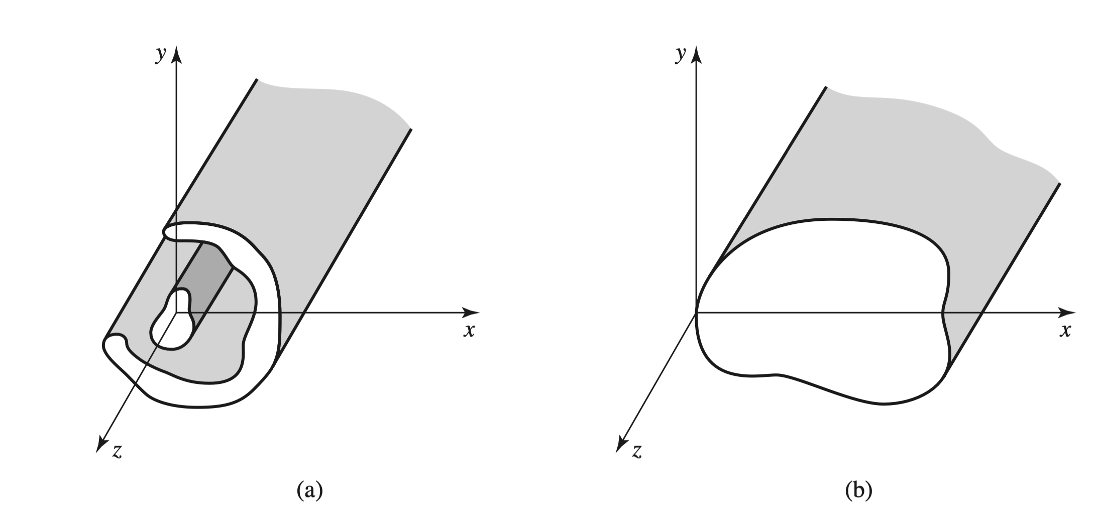
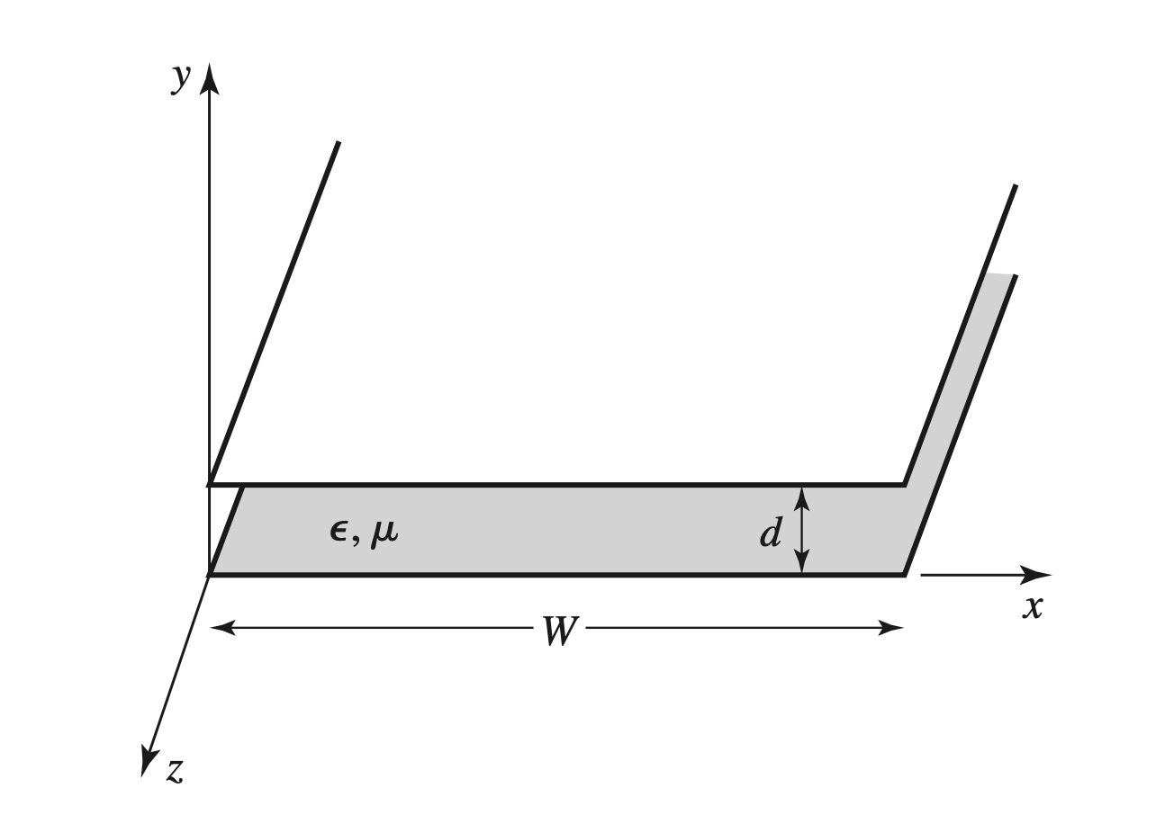
Parallel Plate Waveguide

Image

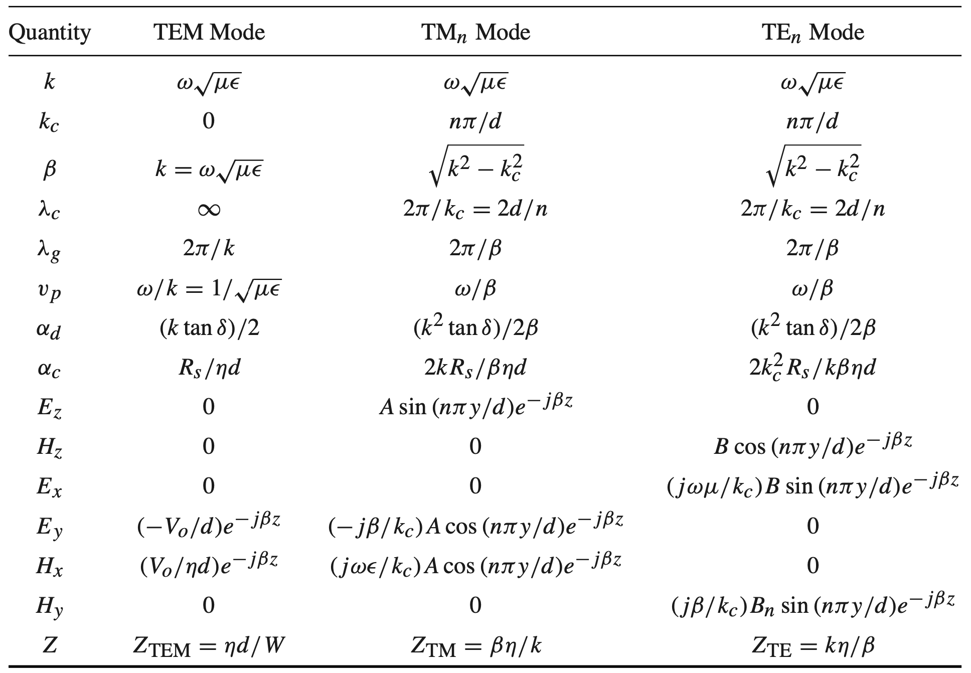
TEM Mode

Voltage Potentials & Transverse Electric Fields

$$ \begin{gather} \begin{aligned} \nabla^2_t \phi(x,y) &= 0 \\ \phi(x, 0) &= 0 \\ \phi(x, d) &= V_0 \\ \therefore \phi(x,y) &= \frac{ V_0 }{ d } y \\ \overrightarrow{ e }(x,y) &= - \nabla_t \phi(x,y) = - \frac{ V_0 }{ d } \overrightarrow{ y } \end{aligned} \end{gather} $$

Fields & Wave Impedance

• $V$和$I$指的是Top Metal的

$$ \begin{gather} \begin{aligned} \overrightarrow{ E } (x,y,z) &= \overrightarrow{ e }(x,y) \cdot e^{-j k z} \\ &= - \overrightarrow{ y } \frac{ V_0 }{ d } e^{-j k z} \\ \overrightarrow{ H }(x,y,z) &= \frac{ 1 }{ \eta } \overrightarrow{ z } \times \overrightarrow{ E } \\ &= \overrightarrow{ x } \frac{ V_0 }{ \eta d } e^{-j k z} \\ V &= - \int_{ y= 0 }^{ d } \overrightarrow{ E }y d \overrightarrow{ y } = V_0 e^{-j k z} \\ I &= \int{ x = 0 }^{ W } \overrightarrow{ H }_x \cdot d \overrightarrow{ x } = \frac{ V_0 W }{ \eta d } e^{-j k z} \\ Z &= \frac{ V }{ I } = \frac{ \eta d }{ W } \end{aligned} \end{gather} $$

TM Mode

Electric Field

• 注意到$\dfrac{ \partial }{ \partial x } = 0$

$$ \begin{gather} \begin{aligned} ( \frac{ \partial^2 }{ \partial y^2 } + k_c^2) e_z(x,y) &= 0 \\ \therefore e_z(x,y) &= A \sin (k_c x) + B \cos (k_c x) \\ e_z(x,y) &= 0, y = 0, d \\ \therefore k_c &= \frac{ n \pi }{ d }, n = 0,1,2,3 \\ \beta &= \sqrt{ k^2 - k_c^2 } \\ \therefore E_z(x,y,z) &= e_z(x,y) \cdot e^{-j \beta z} \\ &= A_n \sin \Big( \frac{ n \pi }{ d } x\Big) \cdot e^{-j \beta z} \end{aligned} \end{gather} $$

• 由此可以得到$E_x, H_x, E_y, H_y$

Wave Impedance& Cutoff Frequency & Wavelength

$$ \begin{gather} \begin{aligned} Z &= -\frac{ E_y }{ H_x } = \frac{ \beta }{ \omega \epsilon } = \frac{ \beta \eta }{ k } \\ f_c &= \frac{ k_c }{ 2\pi \sqrt{ \epsilon \mu } } = \frac{ n }{2d \sqrt{ \epsilon \mu } } \\ \lambda_g &= \frac{ 2\pi }{ \beta } \\ \lambda_c &= \frac{ 2\pi }{ k_c } = \frac{ 2d }{ n } \end{aligned} \end{gather} $$

• 低于$f_c$的叫做Cutoff Mode

Power & Dominant Mode

1. Power

$$ \begin{gather} \begin{aligned} P_o &= \frac{ 1 }{ 2 } \mathcal{Re} \int_{ y= 0 }^{ d } \int_{x = 0 }^{ W } \overrightarrow{ E } \times \overrightarrow{ H }^* \cdot \overrightarrow{ z } dx dy \\ &= \begin{cases} \dfrac{ W \mathcal{Re} ( \beta) \omega \epsilon}{ 2 k_c^2 } |A_n|^2 & n = 0 \\ \dfrac{ W \mathcal{Re} ( \beta) \omega \epsilon}{ 4 k_c^2 } |A_n|^2 & n > 0 \end{cases} \end{aligned} \end{gather} $$

2. Dominant $TM_1$ Mode

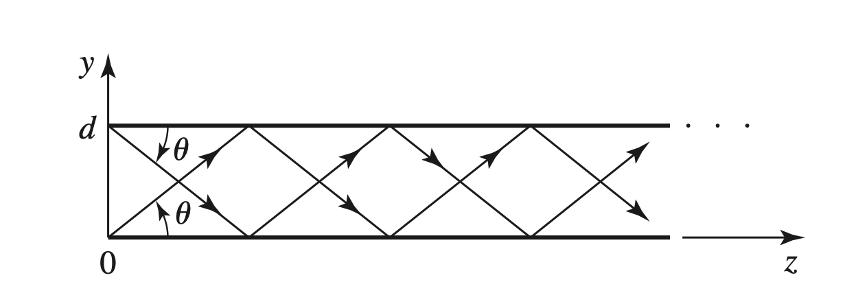
• Electric Field

$$ \begin{gather} \begin{aligned} E_z &= A_1 \sin \Big( \frac{ \pi }{ d } y \Big) e^{-j \beta z} \\ &= \frac{ A_1 }{ 2j } \Big[ e^{j(\pi y /d - \beta_1 z)} - e^{-j ( \pi y/d + \beta_1 z)} \Big] \end{aligned} \end{gather} $$

• Angle $\theta$

$$ \begin{gather} \begin{aligned} ( \frac{ \pi }{ d })^2 + \beta_1^2 &= k^2 \\ k \sin \theta &= \frac{ \pi }{ d } \\ k \cos \theta &= \beta_1 \end{aligned} \end{gather} $$

Dielectric Loss

$$ \begin{gather} \begin{aligned} P_l &= I^2 R_S \\ &= R_s \oint_{ x = 0 }^{ W } H_x \cdot d \overrightarrow{ x } \\ &= \frac{ \omega^2 \epsilon^2 W^2 R_s}{ k_c^2 } |A_n|^2 \\ \therefore \alpha_c &= \frac{ P_l }{ 2P_o } \\ &= \frac{ 2k R_s }{ \beta \eta d } \end{aligned} \end{gather} $$

TE Mode

• 跟TM Mode同理

Summary

Rectangular Waveguide

• 一个导体产生不了TEM Mode

TE Mode

Image

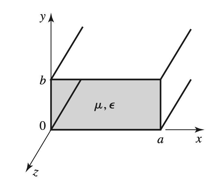
Magnetic Field

$$ \begin{gather} \begin{aligned} 0 &= \Big( \frac{ \partial^2 }{ \partial x^2 } + \frac{ \partial^2 }{ \partial y^2 } + k_c^2 \Big) h_z(x,y) \\ h_z &= X(x) Y(y) \\ h_z(x,y) &= (A \cos (k_x x) + B \cos (k_x y))(C \cos(k_x x) + D \sin (k_y y)) \\ e_x(x,y) &= 0, x = 0, a \\ e_y(x,y) &= 0, y = 0,b \\ \therefore H_z(x,y,z) &= A_{mn} \cos \frac{ m \pi x}{ a } \cos \frac{ n \pi y }{ b } e^{-j \beta z} \end{aligned} \end{gather} $$

Wavelength, Cutoff Frequency, Wave Impedance

$$ \begin{gather} \begin{aligned} f_{c \ mn} &= \frac{ k_c }{ 2 \pi \sqrt{ \epsilon \mu } } = \frac{ 1 }{ 2 \pi \sqrt{ \epsilon \mu } } \sqrt{ ( \frac{ m \pi }{ a })^2 + ( \frac{ n \pi }{ b })^2 } \\ \lambda_g &= \frac{ 2\pi }{ \beta } > \lambda = \frac{ 2 \pi }{ k } \\ Z_{TE} &= \frac{ k \eta }{ \beta } \end{aligned} \end{gather} $$

Dominant Mode Power & Dielectric Loss

• 在$TE_{10}$ Mode 下

$$ \begin{gather} \begin{aligned} P_{10} &= \frac{ 1 }{ 2 } \mathcal{Re} \int_{ x = 0 }^{ a } \int_{ y = 0 }^{ b } \overrightarrow{ E } \times \overrightarrow{ H }^* dx dy \\ &= \frac{ \omega \mu a^3 b |A_{10}|^2}{ 4 \pi^2 } \mathcal{Re} ( \beta) \\ P_l &= R_s \Big[ \Big( \int_{ }^{ } H_x dx\Big)^2 + \Big( \int_{ }^{ } H_y dy \Big)^2 \Big] \\ &= R_S|A_{10}|^2 ( b + \frac{ a }{ 2} + \frac{ \beta^2 a^3 }{ 2 \pi^2 }) \\ \alpha_c &= \frac{ P_l }{ 2P_o } \\ &= \frac{ R_S }{ a^3 b \beta k \eta } (2 b \pi^2 + a^3 k^2) \end{aligned} \end{gather} $$

TM Mode

• 同理

TMm0 Mode in a Partially Loaded Waveguide

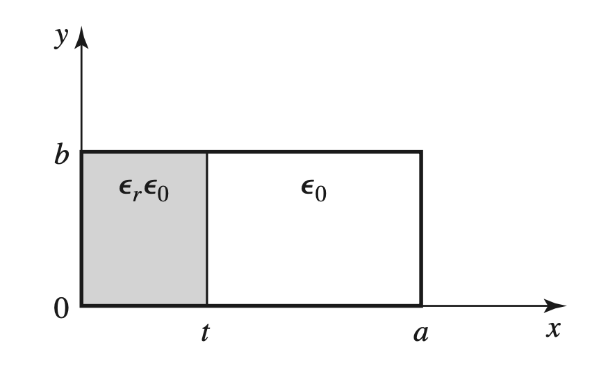
• 电磁波的Phase在Interface上具有连续性

$$ \begin{gather} \begin{aligned} h_z &= \begin{cases} A \cos(k_d x) + B \sin (k_d x) & 0 < x < t\\ C \cos \Big[ k_d(a - x) \Big] + D \sin\Big[ k_d( a- d) \Big] & t < x < a \end{cases} \\ \beta &= \sqrt{ \epsilon_r k^2 - k_d^2 } \\ &= \sqrt{ k^2 - k_a^2 } \end{aligned} \end{gather} $$

• 为了满足Boundary Condition

$$ \begin{gather} \begin{aligned} k_a \cdot \tan (k_d t) + k_a \cdot \tan \Big[ k_a (a - t) \Big] &= 0 \end{aligned} \end{gather} $$

Summary

Circular Waveguide(!!!)

Coaxial Line

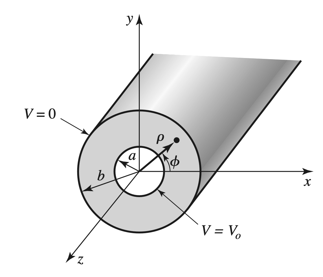
TEM Mode

$$ \begin{gather} \begin{aligned} \nabla^2 \Phi( \rho, \phi) &= 0 \\ \frac{ 1 }{ \rho } \frac{ \partial }{ \partial \rho } \Big( \rho \cdot \frac{ \partial \Phi }{ \partial \rho } \Big) + \frac{ 1 }{ \rho^2 } \Big( \frac{ \partial^2 \Phi}{ \partial \phi^2 } \Big) &= 0 \\ \Phi ( \rho, \phi)&= R( \rho) P( \phi) \\ \therefore \frac{ \rho }{ R } \frac{ \partial }{ \partial \rho } \Big( \rho \cdot \frac{ d^2 R}{ d \rho^2 } \Big) &= - k_{ \rho}^2 \\ \frac{ 1 }{ P } \frac{ d^2 P }{ d \phi^2 } &= -k_{ \phi}^2 \\ k_{ \rho}^2 + k_{ \phi}^2 &= 0 \end{aligned} \end{gather} $$

• 由于Volatge和Angle没有关系, 所以$k_{ \phi}= 0$, 所以$k_{ \phi} = 0$

$$ \begin{gather} \begin{aligned} \Phi( \rho, \phi) &= C ln \rho + D \\ \Phi(a, \phi) &= V_0, \Phi(b, \phi) = 0 \\ \therefore \Phi( \rho, \phi) &= \frac{ V_0 ln(b / \rho)}{ ln(b/a) } \end{aligned} \end{gather} $$

Higher Order Modes

Surface Wave on a Grounded Dielectric Sheet

Image

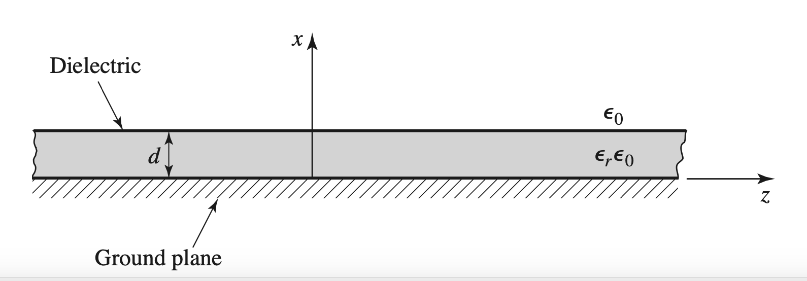
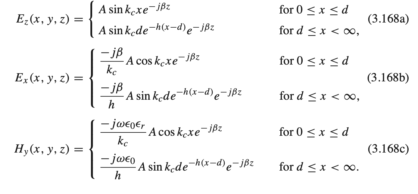
TM Mode

E-Field in Both Medias

$$ \begin{gather} \begin{aligned} k_c^2 &= \epsilon_r^2 k_0^2 - \beta^2 \\ h^2 &= \beta^2 - k_0^2 \\ k_c^2 + h^2 &= ( \epsilon_r + 1) k_0^2 \\ e_z(x,y) &= \begin{cases} A \sin (k_c x) + B (\cos(k_c x)) & 0 < x < d\\ C e^{hx} + D e^{-hx} & x > d \end{cases} \end{aligned} \end{gather} $$

Boundary Condition & Solutions

1. Boundary Condition

$$ \begin{gather} \begin{aligned} \overrightarrow{ E }_z(0, y, z) &=0 \Longrightarrow A =0 \\ \overrightarrow{ E }_z ( \infin , y, z) &< \infin \Longrightarrow C =0 \\ \overrightarrow{ E }_z (d,y,z) \ &Continuous \Longrightarrow A \sin (k_c d) = D e^{-h d} \\ \overrightarrow{ H }_y \ &Continuous \Longrightarrow \frac{ \epsilon_r A }{ k_c } \cos(k_c d) = \frac{ D }{ h } e^{-hd} \end{aligned} \end{gather} $$

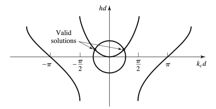
2. Solutions from BC and Propogation Equation

$$ \begin{gather} \begin{aligned} \frac{ k }{ \epsilon_r } \tan (k_c d) &= h \\ \therefore k_c d \tan(k_c d) &= \epsilon_r hd \\ (k_c d)^2 + (hd)^2 &= ( \epsilon_r + 1) (k_0 d)^2 \end{aligned} \end{gather} $$

3. Cutoff Frequency

$$ \begin{gather} \begin{aligned} f_c &= \frac{ nc }{ 2 d \sqrt{ \epsilon_r -1 } } \end{aligned} \end{gather} $$

Field Solutions

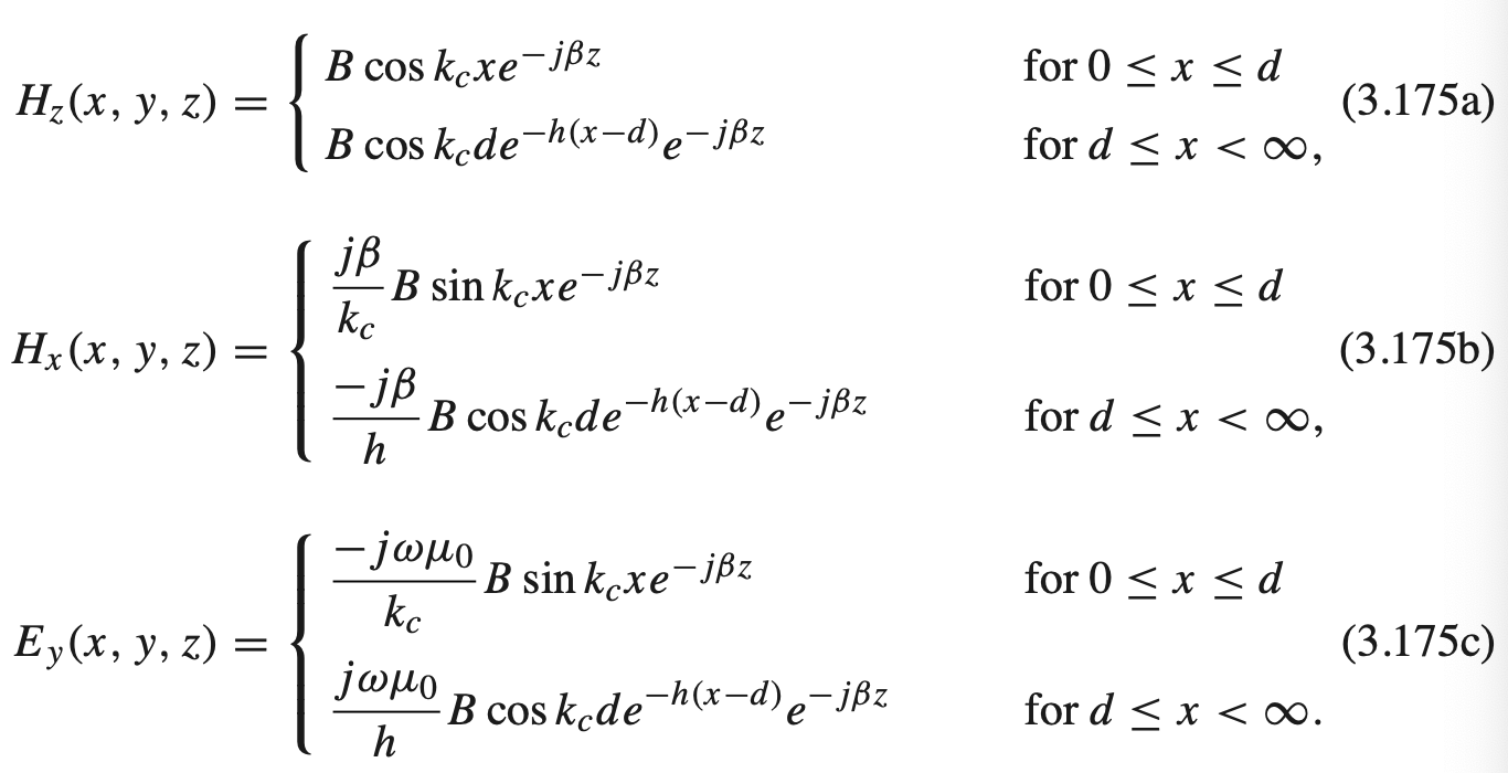
TE Mode

$$ \begin{gather} \begin{aligned} -k_c d \cot (k_c d) &= hd \\ (k_c d)^2 + (hd)^2 &= ( \epsilon_r - 1)(k_0 d)^2 \\ f_c &= \frac{ (2n -1)c }{ 4d \sqrt{ \epsilon_r - 1 } } \end{aligned} \end{gather} $$

Stripline & Microtrip Line

Propogation Coefficient & Impedance

$$ \begin{gather} \begin{aligned} v_p &= \frac{ 1 }{ \sqrt{ \epsilon_r } } \\ \beta &= \frac{ \omega }{ v_p } \\ &= \sqrt{ \epsilon_r } k_0 \\ Z_0 &= \sqrt{ \frac{ L }{ C } } \\ &= \frac{ 1 }{ v_p C } \end{aligned} \end{gather} $$

• 其他的公式感觉暂时用不上，以后再学吧